What is Statistical Inference?
- The primary goal of statistics is to perform statistical inference, which is to deduce the unknown but constant population parameters ($\mu$ or $p$) based on the known but potentially random sample statistics ($\bar{x}$ or $\hat{p}$).
What is Statistical Inference?
- It has two major topics:
- Estimation : What are the probable values of the population parameter? For example, what is $\mu$?
- Hypothesis Testing: Is certain preconception about the population parameter plausible? For example, $\mu = 0$ or not?
Our schedule
We will focus on the inference about population proportion $p$ based on a single sample in this lecture, and the inference about population mean $\mu$ in the next lecture.
And for today's lecture, we will begin by Hypothesis Testing!
The origin of Hypothesis Testing
A famous example described by Ronald Fisher: Lady Tasting Tea.
Who is Ronald Fisher?
A genius who almost single-handedly created the foundations for modern statistical science
YouTubeVideo('lgs7d5saFFc')
Statistical Hypothesis Testing - some basic concept
In statistics, a hypothesis is a statement about a population, usually claiming that a population parameter takes a particular numerical value or falls in a certain range of values.
Null hypothesis ($H_0$, “H-naught”, "H-null", "H-zero" or "H-oh"): a statement that the parameter takes a particular value (or a particular range of values.) This is the hypothesis that we wish to reject.
Statistical Hypothesis Testing - some basic concept
Alternative hypothesis ($H_a$): the opposite of $H_0$. This is the hypothesis that we wish to establish.
A significance test is a method for using data to summarize the evidence about $H_0$ versus $H_a$.
Statistical Hypothesis Testing - an example
- A statistical test procedure is comparable to a criminal trial.
A defendant is considered not guilty as long as his or her guilt is not proven. The prosecutor tries to prove the guilt of the defendant.
Only when there is enough evidence for the prosecution is the defendant convicted.
Statistical Hypothesis Testing - an example
- In the start of the procedure, there are two hypotheses:
- $H_0$: "the defendant is not guilty"
- $H_a$: "the defendant is guilty"
Statistical Hypothesis Testing - three types
- Table 1

Statistical Hypothesis Testing - more details
A test statistic measures how far the sample statistic falls from the null hypothesis value. It is usually in the form of a z-score (in this lecture) or a t-score (in the next lecture).
Assuming $H_0$ is true, the P-value is the probability that the test statistic equals the observed value or a value even more extreme against $H_0$.
Statistical Hypothesis Testing - more details
Comparing the P-value to a predetermined significance level $\alpha$, we make decisions as the following:
- Reject $H_0$ if P-value < $\alpha$;
- Do not reject $H_0$ if P-value ≥ $\alpha$.
The significance level α is usually chosen to be 0.05, 0.10 or 0.01.
Statistical Hypothesis Testing - Remarks
Here are a couple of remarks about interpreting a hypothesis test.
- We draw conclusions (to reject or not to reject) in terms of the null hypothesis $H_0$.
Statistical Hypothesis Testing - Remarks
- Even if the data we have agree with $H_0$, we never “accept” the null hypothesis. Here is the famous criminal trial analogy: suppose that $H_0$ is the defendant being innocent, and $H_a$ the defendant being guilty. If there is not enough evidence to support $H_a$, the judge always concludes that the defendant is “not guilty”, instead of “innocent”.
Statistical Hypothesis Testing - Summaries
Too many concepts and I don't know what the hack are they? 😖
Here is the recipe of doing Hypothesis Testing of popuplation proportion(next slides). 😄
Hypothesis Testing on population proportion - 5 steps
First, set up the null $H_0$ and the alternative $H_a$:
$H_a$ is what we are interested in, and $H_0$ is the opposite of $H_a$;
The hypothesis should have one of the three forms according to Table 1 (Left/Right tail, Two sided).
Hypothesis Testing on population proportion - 5 steps
- Second, Check if $n \times p_0 \geq 15$ and $n \times (1 − p_0) \geq 15$ (recall Chapter 7, CLT).
Hypothesis Testing on population proportion - 5 steps
Third, compute the test statistic $z^*$ through:
$$ z^* = \frac{\hat{p} - p_0}{ \sqrt{ \frac{p_0(1-p_0)}{n} }} $$
Fourth, compute the P-value based on the $z^∗$ according to Table 2.
Hypothesis Testing on population proportion - 5 steps
- Fifth, draw conclusion by comparing the P-value to the significance level α.
- If P-value < $\alpha$, --> reject $H_0$. There is sufficient evidence to support $H_a$ under $\alpha$ significance level.
- If P-value ≥ $\alpha$, --> do not reject $H_0$. There is no sufficient evidence to support $H_a$ under $\alpha$ significance level.
Hypothesis Testing - practice
- Let's practice how to do hypothesis testing!
Confidence Interval - preliminary
What is confidence interval?
We use sample proportion $\hat{p}$ to estimate $p$. $\hat{p}$ is called the point estimate for the population proportion.
An interval estimate is an interval of numbers that is believed to contain the actual value of the parameter.
Confidence Interval - preliminary
- Remark: representing the population parameter by a single number we obtain from a single sample does not take into consideration the random nature of a sample. In this sense, an interval estimate is much more reasonable.
Confidence Interval
A confidence interval (CI) is an interval estimate containing the most believable values for a parameter.
It is formed by combining the point estimate and a margin of error (more details in next slide).
Confidence Interval
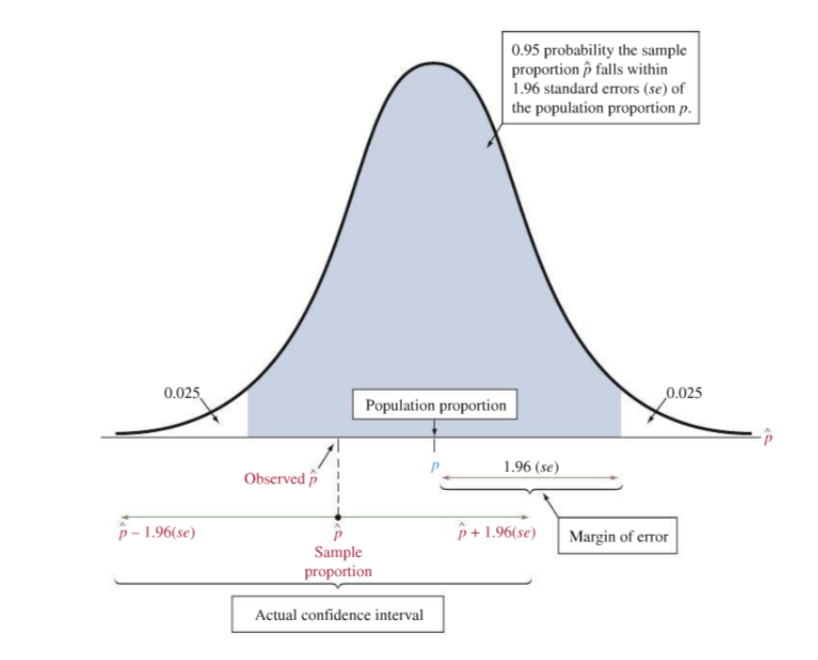
The probability that this method produces an interval that contains the parameter is called the confidence level.
Confidence level is a number less than 1 that we subjectively choose before constructing the interval. Common choices for confidence level are 0.95 (95%), 0.90 (90%) or 0.99 (99%).
Confidence Interval for sample proportion - 6 steps
- Find the sample proportion pb. This is usually given, or can be easily computed through
Confidence Interval for sample proportion - 6 steps
- Check the following two assumptions:
- $n \times \hat{p} \geq 15$
- $n \times (1 − \hat{p}) \geq 15$
Confidence Interval for sample proportion - 6 steps
- Compute the standard error (se) through $$ se = \sqrt{ \frac{\hat{p}(1-\hat{p})}{n} } $$
Confidence Interval for sample proportion - 6 steps
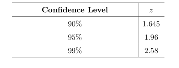
Find the correct z-score according to the given confidence level from Table 3, then compute the margin of error (MOE) through $$ MOE = z \times se$$
The lower limit (LL) of the CI is $$ \hat{p} - MOE$$ and The upper limit (UL) of the CI is $$ \hat{p} + MOE$$
Hence the desired ci is given by $(LL, UL)$.
Interpretation: We are ...% confident that the interval (LL, UL) covers the population proportion $p$.
Confidence Interval for sample proportion - 6 steps
- Table 3

Confidence Interval for sample proportion - the formula
- CI for population proportion in one line: $$ \big( \hat{p} - z\sqrt{ \frac{\hat{p}(1-\hat{p})}{n} }, \hat{p} + z\sqrt{ \frac{\hat{p}(1-\hat{p})}{n} } \big) $$
Confidence Interval - illustarated

Confidence Interval - Remark
- As we lower the confidence level, margin of error decreases, and hence the confidence interval becomes narrower.
Our schedule - Updated
Recall last week, we did the one sample inference about population proportion $p$
We will talk about one sample inference about population mean $\mu$ today, especially in the case where we do not have a large sample ($n < 30$).
Review
Recall from Chapter 7, by the Central Limit Theorem (CLT), if we have a sample of size $n \geq 30$ from any population with unknown parameters mean $\mu$ and standard deviation $\sigma$, the sampling distribution of the sample mean $\bar{X}$ is
$$ \bar{X} \sim \mathcal{N}(\mu, \frac{\sigma}{\sqrt{n}})$$
Or equivalently, $$ \frac{\bar{X} - \mu}{\sigma / \sqrt{n}} \sim \mathcal{N}(0, 1) $$
Review
Actually, we can use the fact $ \frac{\bar{X} - \mu}{\sigma / \sqrt{n}} \sim \mathcal{N}(0, 1) $ to make statistical inference, but
- We don't know the true value of $\sigma$.
- We need large sample size.
What will we do then ?
For a normally distributed population with population mean $\mu$, a random sample of size $n$ from this population with sample mean $\bar{X}$ and sample standard deviation $s$, we have the expression (t-score) $$t = \frac{\bar{X} - \mu}{s / \sqrt{n}}$$
follows Student’s t-distribution with $(n − 1)$ degrees of freedom ($df$).
- Or equivalently $$ t=\frac{\bar{X} - \mu}{s / \sqrt{n}} \sim T(n-1) $$
T-distribution

Properties of t-distribution
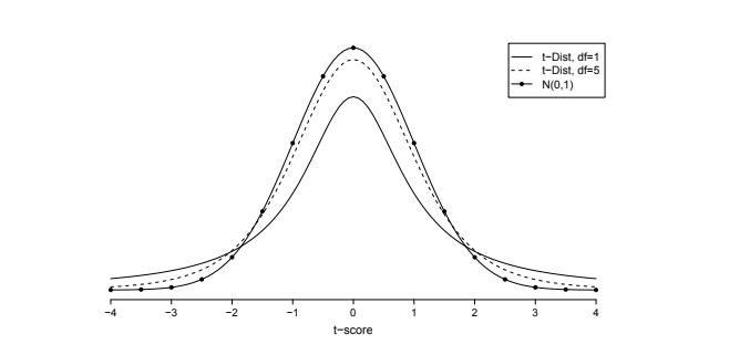
Like the standard normal distribution, t-distribution is bell-shaped and symmetric about 0.
The shape of the density curve of t-distribution varies for each distinct value of df. Probabil- ities and t-scores depend on the specific value of df, i.e. on the sample size.
Properties of t-distribution
Comparing to the standard normal distribution, t-distribution has more density at the tails, and hence more variability. This is caused by replacing the fixed quantity σ with the random quantity S. However, as the sample size n increases, the shape of t-distribution gradually approaches that of a standard normal distribution.
The t-Distribution Table (or t-table for short) lists t-scores for certain values of right-tail probabilities and df. We use tα to denote the t-score that has a right-tail probability α. For instance, for $df = 1$, $t_{.100} = 3.0784$. This means $P(t > 3.078) = .100$.
Why it is call student's t distribution?
- A historical note: the name “Student’s t-distribution” comes from the early 20th century statistician William Gosset, who spent much of his career as a chemist in the Guinness Breweries, in the mean time publishing research papers under the pseudonym “Student”.
T-table
- On the appendix of your text book Statistics: The art and science of learning from data
IFrame("https://statcao.github.io/teaching/t-table.pdf", width=800, height=600)
Confidence interval for the population mean
Recall from the last lecture that the confidence interval (CI) for a population parameter is a collec- tion of the most probable values of that parameter, and is of the form
point estimate ± margin of error
Confidence interval for the population mean - the recipe
CI for the population mean $\mu$, the point estimate is the sample mean $\bar{x}$, and the margin of error is the standard error multiplied by a t-score.
Suppose we have a random sample of size $n$ with mean $bar{x}$ and standard deviation $s$, ...
Confidence interval for the population mean - the recipe
- First, check the following assumptions:
- The observations must be quantitative.
- If $n \geq 30$, go to the second step. Otherwise, continue checking.
- If $ n < 30 $, then the observations must be normally distributed. (This is usually assumed to be true.)
Confidence interval for the population mean - the recipe
- Second, compute the standard error (se) through $$ se = \frac{s}{\sqrt{n}}$$
Confidence interval for the population mean - the recipe
Third, find the t-score from the t-table according to the given confidence level and $df = n−1$. Then, compute the margin of error (MOE) through $$ MOE = t \times se $$
Fouth, the CI is given by
$$CI = (\bar{x} − MOE, \bar{x} + MOE)$$
Fifth, the interpretation: we are ...% confident that the population mean is in between $\bar{x} − MOE$ and $\bar{x} + MOE$.
Hypothesis tesing on sample mean
A hypothesis test that utilizes the t-distribution is usually referred to as a t-test.
Suppose we have a sample of size $n$ with sample mean $\mu$ and standard deviation $s$.
Hypothesis tesing on sample mean - the recipe
- First, check the following assumptions:
- The observations must be quantitative.
- If $n \geq 30$, go to the second step. Otherwise, continue checking.
- If $ n < 30 $, then the observations must be normally distributed. (This is usually assumed to be true.)
Hypothesis tesing on sample mean - the recipe
- Second, set up $H_0$ and Ha according to the table below. $H_a$ is the hypothesis of interest that the population mean $\mu$ is within a particular range associated with some pre-conceived $\mu_0$, and $H_0$ is the opposite of $H_a$.

Hypothesis tesing on sample mean - the recipe
Third, compute the test-statistic t^∗ through
$$t^* = \frac{\bar{x} - \mu_0}{s / \sqrt{n}}$$
Hypothesis tesing on sample mean - the recipe
- Fouth step (the hard way), Based on $t^∗$ a given significance level $\alpha$, make a decision by comparing $t^∗$ to a certain t-score which we call critical value from the t-table.

- The table provides the conditions for rejecting $H_0$ under the three different types of $H_a$. If the condition in the last column is not satisfied, we fail to reject $H_0$.
Hypothesis tesing on sample mean - the recipe
- The table in previous slides looks scary, other approaches available? --- YES
Hypothesis tesing on sample mean - another forth step
- Forth step (the easier way), calculate p-value using statistical software (Stat Crunch, for this course).
Hypothesis tesing on sample mean - the recipe
- Fifth, draw conclusion by comparing the P-value to the significance level α.
- If P-value < $\alpha$, --> reject $H_0$. There is sufficient evidence to support $H_a$ under $\alpha$ significance level.
- If P-value ≥ $\alpha$, --> do not reject $H_0$. There is no sufficient evidence to support $H_a$ under $\alpha$ significance level.
