Recall what is sample, what is sample statistic
Sample: A subset of the population, a collection of individuals that we have data.
(Sample) statistic: A nummerical summary of the sample, such as sample mean $\bar{x}$, sample standard deviation $s$.
What is sampling distribution?
The sample statistic, i.e., $\bar{x}$, s, etc. also has a probability distribution!
The sample distribution of a statistic is the probability distribution that specifies probabilities for the possible values the statistic can take.
Sampling distribution: more detail
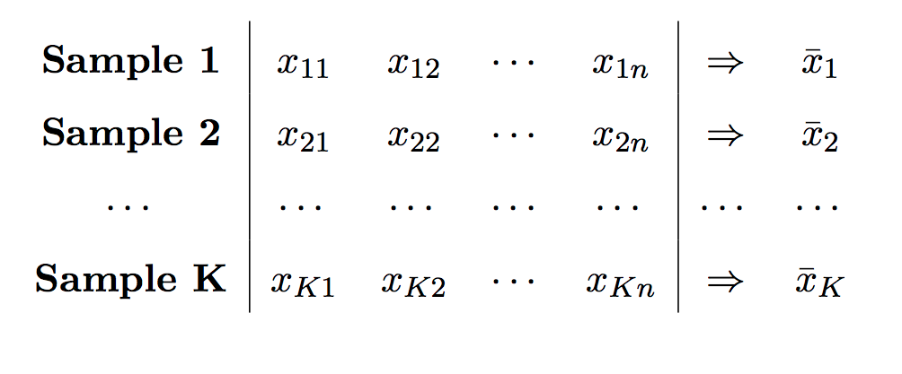
- Suppose we were able to collect $K$ different random samples, each of size $n$, from the same population, and to compute the sample mean $\bar{x}$ for each random sample:

Sampling distribution: more detail
Hence, we could further plot the $\bar{x}$'s as, say, a histogram. In other words, we could obtain an entire distribution for the random sample mean $\bar{x}$.
However, the exact sampling distribution of $\bar{x}$ is usually difficult to obtain, and collecting multiple samples is usually infeasible in reality.
Sampling distribution of $\bar{x}$ - A special case
- For a random sample of size $n$ from a normal population with mean $\mu$ and standard deviation $\sigma$, the sampling distribution of the sample mean $\bar{x}$ is
- The standard deviation in the sampling distribution, $\frac{\sigma}{\sqrt{n}}$, is usually referred to as the standard error.
Sampling distribution of $\bar{x}$ - A general case
In the previous slides, we assume the random sample are drawn from a normal distribution. What aboout other distributions?
For a general case, this is refered to the Central Limit Theorm (CLT).
Central Limit Theorem
- For a random sample of size $n$ from a population with mean $\mu$ and standard deviation $\sigma$, if the sample size is large enough, then, the sampling distribution of the sample mean $\bar{x}$ is approximately
Central Limit Theorem - simulation
IFrame("http://47.254.76.4:3838/sample-apps/CLT_demo/", width=800, height=600)
Central Limit Theorem - Rule of a thumb
- How large is large enough for the sample size $n$?
- Rule of a thumb: $n \geq 30$
Sample proportion $\hat{p}$
- Recall sample proprotion is defined via:
The number of observations falling in one category divided by the total number of observations. In other words, sample proportion is the frequency of one category divided by the sample size. We often denote sample proportion by $\hat{p}$ (p-hat).
Sampling distribution of $\hat{p}$
For a random sample of size $n$ which satisfies the following conditions:
- the observations are binary ($successes$ or $failures$) with $P(success) = p$
n is large enough, or more specifically $np \geq 15$ and $n(1 − p) \geq 15$ (rule of thumb)
then, the sampling distribution of the sample proportion of successes $\hat{p}$ is approximately
$$ \hat{p} \sim \mathcal{N} \big(p, \sqrt{\frac{p(1-p)}{n}} \big) $$
Sampling distribution of $\hat{p}$ - some remarks
This result is an application of CLT. Each observation in the population has a $binomial(1, p)$ distribution with mean $\mu = p$ and standard deviation $\sigma = \sqrt{p(1 − p)} $.
The exact probability distribution of $\hat{p}$ is discrete.
Sampling distribution - simulation
IFrame("http://47.254.76.4:3838/sample-apps/sample_proportion_CLT/", width=800, height=600)