Randomness -- flip a coin
A phenomenon is a random phenomenon if all possible outcomes of the phe- nomenon are known, but which one occurs is uncertain. We use probability to quantify the uncer- tainty in random phenomena.
A random trial or random experiment is any observable action in which the occurrence of the outcomes is random.
Random Noise

Which one is more "random" ?
- Suppose you flipped a coin many times, H means you observed a head, T means tail.
- Two records:
- HTTHTTTHTTTHHTTTTHTHTTHHHTHTHTTHHHHTHHHHTTHHHHHHHHHTH THTHTHTTHTHTHHHTHHTHTTHHTTHHTHTHHTHHTHTTTTHTTHH
- HTTHTHTHTTHTHHTHTTHTHTTHTTTHTTHTTTHTTHTHTTHTHTTHTTTHT HTHTHTTHTHTHHTHTHTHTHTHTHTHTHTTHTHTHTTTHTTHTTHT
Probability
The probability of an event A is the proportion of times that the event occur in a long run of observations. We often denote the probability of an event A by $P(A)$.
Remark. The above definition is usually referred to as the law of large numbers (LLN), which states that the sample proportion of an event A gradually approaches P(A) as the sample size n increases to infinity.
LAW of Large Numbers
Sample space and Events
- The sample space of a random trial, denoted by S, is the collection of all possible outcomes of the trial.
- An event is a sub-collection of some outcomes within the sample space.
Calculating the probability
- In case the number of outcomes in S is finite, if the outcomes are all equally likely to occur, then the probability of an event A is given by
Basic properties
$P(S) = 1$
For any event $A$, $0 ≤ P(A) ≤ 1$
- If $P(A) = 1$, we call the event $A$ a sure event.
- If $P(A) = 0$, we call the event $A$ an impossible event.
The probabilities of all outcomes should sum to 1.
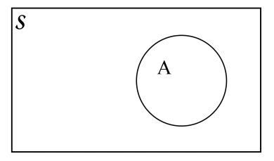
Venn diagram
- A Venn diagram, displays the relationship between a
sample space and possible events, in which
- the rectangle represents the sample space S;
- the circle represents a specific event A.

Basic probability rules
- Complement $A^c$: all outcomes in the sample space $S$ that do not belong to the event $A$.
- Disjoint events: two events, $A$ and $B$, are disjoint if they do not share any common outcomes. If events $A$ and $B$ are disjoint,
Basic probability rules
- Intersection $A$ and $B$: all outcomes in the sample space S that belong to both $A$ and $B$.
- Union $A$ or $B$: all outcomes in the sample space S that belong to both $A$ or $B$.
Basic probability rules
If events A and B are disjoint, then we have
$$ P(A \operatorname{and} B) = 0 $$
$$ P(A \operatorname{or} B) = P(A) + P(B) $$
Basic probability rules - explained by Venn diagram
- Intersection
Basic probability rules - explained by Venn diagram
- Union
Exercise time!
Conditional probability
For events $A$ and $B$, the conditional probability of event $A$ given that event $B$ has occurred is
$$ P(A | B) = \frac{P(A \operatorname{and} B)}{P(B)} = \frac{\operatorname{Number of outcomes in} A \operatorname{and} B}{\operatorname{Number of outcomes in} B} $$
$P (A|B)$ is read as “the probability of event A given event B”. The pipe “|” represents the word “given”.
The formula above can alos be written as : $$ P(A \operatorname{and} B) = P (A|B) · P(B) = P (B|A) · P(A) $$
Independence
Two events A and B are statistically independent if the occurrence of one event is not affected by whether the other event has already occurred.
$A$ and $B$ are statistically independent if one of the following is satisfied:
- $$ P(A | B) = P(A) $$
- $$ P(B | A) = P(B) $$
- $$ P(A \operatorname{and} B) = P(A) · P(B) $$
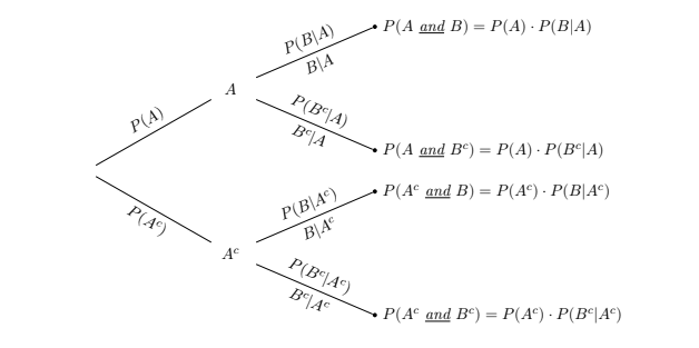
Tree diagram
- We can summarize the probabilities of two events A and B into a tree diagram. The process of creating a tree diagram is as the following:

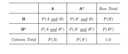
2 - by - 2 contigency table
- Further, we can arrange the intersection probabilities into the 2 × 2 contingency table below.

Clinical example
In clinical studies, an individual has a true identity of whether or not s/he has a certain disease. At the same time, a medical test on the blood sample (or any other sample) taken from the individual can be positive or negative. Let events
$D$ = the individual has the disease
$D^c$ = the individual does not have the disease
$+$ = the test result is positive
$-$ = the test result is negative
Clinical example
Then we have the following terminologies:
The prevalence of a disease, $P(D)$, is the probability of the disease, or how popular the disease is among a group of people.
The sensitivity of a medical test, $P(+|D)$, is the probability of a positive test result given the individual actually has the disease.
The specificity of a medical test, $P(−|D^c)$, is the probability of a negative test result given the individual actually does not have the disease.
Some other terminologies:
| Events | $D$ | $D^c$ | |
|---|---|---|---|
| $+$ | True Positives | False Positives | |
| $-$ | False Negatives | True Negatives |