Association
- An association exists between two variables if particular values of one variable
and particular values of the other variable are likely to occur together.

- Response variable (Dependent Variable)
- the outcome variable on which comparisons are made
- Explanatory variable (Independent variable)
- defines the groups to be compared with respect to values on the response variable
Contigency table - visualize two categorical variables
- Its rows list the categories of one variable.
- Its columns list the categories of the other variable.
- Its entries (cells) are the frequency, i.e. the number of observations that fall in both categories.
In [69]:
Out[69]:
Regression -- association between two quantitative variables
Scatter plot - visualize two quantitative variables
- If we have two quantitative variables, we can graphically display the two variables
using a scatter plot on the x-y plane, where
- the explanatory variable is on the horizontal axis (x-axis)
- the response is on the vertical axis (y-axis)
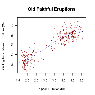
Example: Old Faithful Geyser in Yellowstone National Park.
- Variables:
- Waiting time between eruptions (Response)
- Duration of the eruption (Explanatory)

Scatter plot

Scatter plot
We use the scatter plot to examine three aspects of the association between the two variables:
- Trend (pattern): linear, curved, no pattern, etc.
- Direction: positive, negative, no direction
- Positive: as X increases, Y increases
- Negative: as X increases, Y decreases
- No direction: the increases in X does not affect Y (no association)
- Strength: how closely the points fit the trend
Scatter plot
- In general, we care about whether there is linear trend between the two variables.
- How to measure linear trend ?
Correlation coefficient
- We can measure the strength of linear association between two variables using the correlation coefficient, denoted by $r$.
Basic properties of correlation coefficient $r$
- −1 ≤ r ≤ 1
- If r > 0, there is a positive association between X and Y - Y increases as X increases
- If r < 0, there is a negative association between X and Y - Y decreases as X increases
- The closer r is toward 1 or −1, the stronger the evidence of linear association is.
- The closer r is toward 0, the weaker the evidence of linear association is.
Correlation coefficient 𝑟
- Noticed in the last row, there exist some curved association between X and Y, but the correlation coefficient is 0.
- This is because, correlation coefficient can only measure linear association.
Predicting the Outcome of the Response - regression line
- A regression line predicts the value for the response variable Y as a straight-line function of the value X of the explanatory variable.
Regression line
Let $\hat{y}$ (y-hat) denote the predicted value (fitted value) of the response y, and x the explanatory variable. The equation of the regression line is given by
$$\hat{y} = a + bx $$
- where
- a is the y-intercept: the predicted value of y when x = 0. When it is not meaningful to assign x = 0 to the explanatory variable, a does not have a specific meaning.
- b is the slope: the average increase in the response y as the explanatory variable x increases
by 1 unit.
- If b > 0, there is a positive linear association between X and Y .
- If b < 0, there is a negative linear association between X and Y .
Residual
- Residual is defined as: $$ Residual = y - \hat{y}$$
- Residual can be viewed as the error in prediction.
How do we get the regression line?
- A common procedure to find the regression line is called the least-squares method.
- Using the least-squares method, the regression line always provides the smallest amount of total prediction error, which is called the residual sum of squares.
How do we measure the performance of regression line?
- $R^2$ (R-squared) measures how well the regression line fits the data.
- $R^2$ is defined as $$R^2 = \frac{Variability\ in\ Y\ explained\ by\ regression}{Total\ variability\ in\ Y}$$
which is the proportion (percentage) of the variability in Y explained by the the regression.
$R^2$ and $r$
- Connection between R-squared $R^2$ and correlation coefficient $r $:
- If $b>0$, $ r = \sqrt{R^2}$
- If $b<0$, $ r = -\sqrt{R^2}$
- Recall $b$ is the slope in the regression line
Cautions in Regression
- Extrapolation – using linear regression to make predictions for values of x that are outside of the range of collected data is risky.
- Influential outliers
In [73]:
import matplotlib.pyplot as plt
%matplotlib inline
import numpy as np

X = np.random.rand(100)
Y = X + np.random.normal(0,1,100)/10

X = np.append(X, 10).reshape(101,1)
Y = np.append(Y, 0.4).reshape(101,1)

from sklearn.linear_model import LinearRegression
regr = LinearRegression().fit(X,Y)
y_pred = regr.predict(X)


plt.scatter(X,Y)
plt.plot(X,y_pred, "r")
Out[73]:
- Correlation does not imply causation
- Famous example: People observed, as the sales of ice cream go up, the incidents of drowning go up as well.
- Does this means ice cream causes drowning ?
In [70]:
Out[70]: