Elmentary Statistics (STAT 201)¶

Xiangyang Cao, PhD candidate in Statistics¶

What is Statistics?¶

Let data tell a story -> The art and science of learning from data¶

• One story: searching for a fisherman lost at sea using Statistics method

• There are two fishermen on a boat in the middle of the night. While one is asleep, the other falls into the ocean. The boat continues to troll along on autopilot all through the night until the first guy finally wakes up and notifies the Coast Guard.

• A long version

Basic concepts in Statistics¶

• Individuals (subjects): the entities that we measure in a study. Individuals are often people, but they don’t have to be.

• Variable: any characteristic we measure on the individuals. The measurements are called data or observations.

  • Values of the same variable may differ among individuals. We call this difference variability.

• Population: the collection of all individuals that we are interested in.
• Sample: a subset of the population which we have (or plan to have) data.
  • The number of individuals in the sample is called the sample size.

• Parameter: a numerical summary of the population, such as population mean or population proportion.
  • Unless every individual in the population is measured, the population parameter is usually unknown.
• Statistic: a numerical summary of the sample, such as sample mean or sample proportion.
  • Although always known, a key feature of a sample statistic is that it is random. The value of a sample statistic varies from sample to sample.

Population vs sample, parameter vs statistic¶

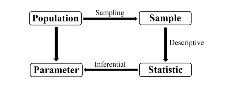
Three main components of statistics:¶

• Design of study: stating the goal and/or question of interest and planning how to obtain data that will address them.

• Descriptive statistics: summarizing and analyzing the data that are obtained.

• Inferential statistics: making decisions and predictions based on the data for answering the statistical question.

Design of study - Sampling Method¶

Scheme	Defination	Pros	Cons
Census	Measureing every individual in the population	Comprehensive	non-feasible
Judgment Sample	A sample that an expert thinks to be representative		Potentially biased
Convenience Sample	A sample that is easy to access		Potentially biased
Volunteer Sample	A sample where individuals choose to/not to participate		Potentially biased
Systematic Sample	Individuals are sampled using systematic methods		Potentially biased
Simple Random Sample(SRS)	Every individual in the population is equally likely to be included in the sample	Represents the population if the sample size is large enough

Data Visualization (Graphical Display)¶

Categorical Data¶

• Categorical (qualitative) : each observation belongs to one of a set of distinct categories.
  • Major, home state, nationality, etc.
  • (There are 10 types of people, those who understand binary system and those who don’t.)

Quantitative Data¶

• Quantitative: each observation takes on a numerical value that represent a certain magni- tude of the variable.

  • Discrete quantitative: possible values of the variable form a set of separate numbers such as 0, 1, 2, . . ..
  • Continuous quantitative: possible values of the variable form an interval.

How to visualize categorical data¶

• Distribution The distribution of a variable describes how the observations fall (are dis- tributed) across the range of possible values.

Frequency table¶

• The distribution of a categorical variable can be summarized in a frequency table, which displays all possible categories, together with the frequencies or relative frequencies of each category.

  • Frequency: the number of observations (or occurrences) falling in one category.
  • Relative frequency: the number of observations falling in one category, relative to the sample size.

• We can obtain the relative frequency of a category by computing its sample proportion or percentage.

• Sample proportion: the number of observations falling in one category divided by the total number of observations. In other words, sample proportion is the frequency of one category divided by the sample size. We often denote sample proportion by $\hat{p}$ (p-hat).

$$ \hat{p} = \frac{frequency}{sample \ size} $$

• An example: number of car accidents in each state in 2017

Pie chart¶

• The earliest pie chart ever created dates back to 1801 (From Wikipedia):

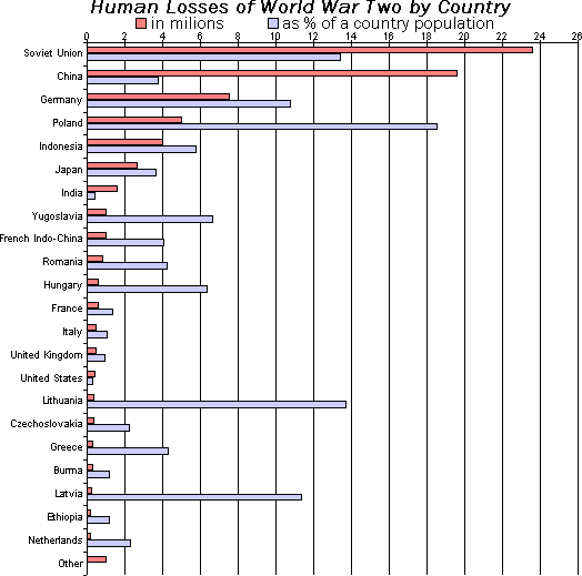
Bar graph¶

• Huamn losses in WWII (From Wikipedia)

How to visualize quantitative data¶

Dot plot¶

• From Wikipedia

Stem and Leaf plot¶

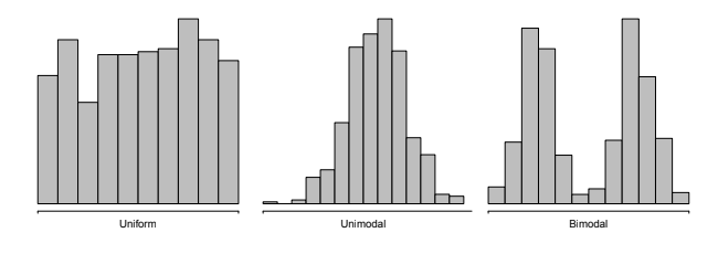
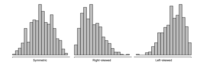
Histogram¶

• Important

• Different shpae of histogram

Boxplot¶

• Important, we will talk about it later.

• Boxplot of the Michelson–Morley experiment (measuring the speed of light) (From Wikipedia)

Descriptive Statistics (Numerical Summary)¶

Measure of Center -- where the “center” of the data is located.¶

• Sample mean
• Sample median

Sample mean¶

• Sample mean: denoted by $\bar{x}$, suppose we have $n$ observations $x_1, x_2, \dots, x_n$

$$\bar{x} = \frac{x_1 + x_2 + \dots + x_n}{n} = \frac{\sum x_i}{n}$$

Sample median¶

• Sample median: midpoint of the observations when they are ordered from the smallest to the largest.
• Calculation:
  1. Sort the observations from the smallest to the largest.
  2. If the sample size, n, is
     • odd, the median is the middle observation;
     • even, the median is the average of the two middle observations.

Sample median¶

• Calculation:
  1. Sort the observations from the smallest to the largest.
  2. If the sample size, n, is
     • odd, the median is the middle observation;
     • even, the median is the average of the two middle observations.

Remark¶

• if the distribution is symmetric, median ≈ mean;
• if the distribution is left-skewed, median > mean;
• if the distribution is right-skewed, median < mean.

Measure of Variability -- how much the data varies¶

• Range, Vairance and Standard deviation

Range¶

• Range = Maximum - Minimum

Variance and standard deviation¶

• Variance: denoted by $s^2$: $$ s^2 = \frac{\sum (x_i - \bar{x})^2}{n-1} $$
• Standard deviation: denoted by $s$: $$ s = \sqrt{s^2} $$

Remark¶

• Like sample mean and median, range, variance and standard deviation are sample statistics. Here for simplicity, we use variance instead of a more rigorious term "sample variance".

Five number summary¶

• We usually refer to the minimum (smallest observation), the first quartile, the median, the third quartile and the maximum (largest observation) as the five-number summary.

First (Q1) and third quartile(Q3)¶

• Sorting the data in ascending order from the smallest to the largest, the first quartile (Q1), the median (second quartile, Q2) and the third quartile (Q3) divide the whole data set into 4 sections, each containing 25% of all the observations.

First (Q1) and third quartile(Q3)¶

1. Sort the data in ascending order from the smallest to the largest.
2. Find the median (Q2) of the whole data set.
3. Exclude Q2. (Not necessary if the sample size n is even.)
4. The median of the lower half of the observations is the first quartile Q1.
5. Similarly, the median of the upper half of the observations is the third quartile Q3.

Recall Boxplot?¶

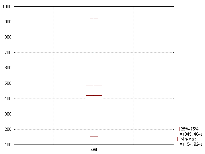
Five number summary and Box plot¶

|--------|二二二二|二二二二|------|

↑        ↑      ↑       ↑      ↑
minmum   Q1     Q2      Q3   maximum

z-score¶

• z-score of an observation $x$: the number of standard deviations $s$ from that observation $x$ to the mean $\bar{x}$. For an observation x, its z-score $z$ is given by

$$ z = \frac{x - mean}{standard\ deviation} = \frac{x - \bar{x}}{s}$$

The empirical rule¶

• For bell shaped (sysmetric) data . . .
  • About 68% of observations fall within 1 standard deviation of the mean, $\bar{x}-s$ to $\bar{x}+s$
  • About 95% of observations fall within 2 standard deviations of the mean, $\bar{x}-2s$ to $\bar{x}+2s$
  • About 100% of observations fall within 3 standard deviations of the mean, $\bar{x}-3s$ to $\bar{x}+3s$

The empirical rule¶

• In terms of z-scores, empirical rule corresponds to
  • 68% of all the observations have −1 < z < 1;
  • 95% of all the observations have −2 < z < 2;
  • 99.7% (100%) of all the observations have −3 < z < 3.

END¶