Introduction
- In the last two lectures, we discussed statistical inference on a population parameter based on a single sample.
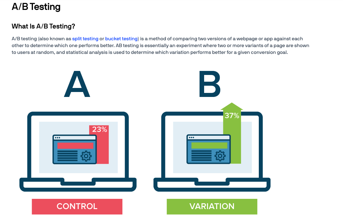
- However, oftentimes we are interested in comparing two different populations. In this lecture, we will focus on inference about the difference between two population means based on two samples taken respectively from each population.
Two sample inference -- an example

The big picture

Comparing two population means
We will start with dependent samples first
The relationship between two samples is either independent or dependent. Thetwo samples are independent if individuals in each sample are completely independent or unrelated.
Independent samples -- an example
- In clinical trials, individuals in the treatment group (sample A) and individuals in the placebo group (sample B) are independent.
- In political surveys, Democrats (sample A) and Republicans (sample B) are independent.
Dependent samples -- defination
- The two samples are dependent (matched pairs) if individuals in both samples either are the same or match each other.
Dependent samples -- an example
In Lab 9, we measure the heart rate of the same individuals before (sample A) and after (sample B) the exercise.
In a study of individuals’ age at marriage, husbands (sample A) and wives (sample B) are matched pairs.
What should we do if we have dependent samples?
If the two samples are dependent, we can take the difference between the matched pairs
And then perform one-sample inference (confidence interval or t-test) on the difference. (Paired t-test)
The differences are usually assumed to be normally distributed. We can check this by looking at a histogram.
Hypothesis tesing on two population means with dependent samples - the recipe
- First, check the following assumptions:
- The sample of difference scores is a random sample from a population of such difference scores
- The difference scores have a population distribution that is approximately normal. This is important for small samples (less than about 30). If the sample size is small ($<30$), make a graphical display and check for extreme outliers or skew.
Hypothesis tesing on two population means with dependent samples - the recipe
- Second, set up the hypothesis.
or $$ \operatorname{Right\ tail:} H_a: \mu_d = \mu_1-\mu_2 > 0, $$ or $$ \operatorname{Two\ sided:} H_a: \mu_d = \mu_1-\mu_2 \neq 0 $$
Hypothesis tesing on two population means with dependent samples - the recipe
Third, compute the test-statistic $t^∗$ through
$$t^* = \frac{\bar{x}_d - 0}{s_d / \sqrt{n}}$$
where $\bar{x}_d$ and $s_d$ are the sample mean and sample standard deviation of the differences, respectively.
$df = n-1$
Hypothesis tesing on twp population means with dependent samples - the recipe (the hard way)
- Fourth step (the hard way), Based on $t^∗$ a given significance level $\alpha$, make a decision by comparing $t^∗$ to a certain t-score which we call critical value from the t-table.

- The table provides the conditions for rejecting $H_0$ under the three different types of $H_a$. If the condition in the last column is not satisfied, we fail to reject $H_0$.
Hypothesis tesing on two population means with dependent samples - the recipe (the easier way)
Fourth step (the easier way), calculate p-value using statistical software (Stat Crunch, for this course).
Fifth, draw conclusion by comparing the P-value to the significance level α.
- If P-value < $\alpha$, --> reject $H_0$. There is sufficient evidence to support $H_a$ under $\alpha$ significance level.
- If P-value ≥ $\alpha$, --> do not reject $H_0$. There is no sufficient evidence to support $H_a$ under $\alpha$ significance level.
Confidence interval for the population mean difference with dependent sample- the recipe
Suppose $\bar{x}_d$ and $s_d$ are the sample mean and sample standard deviation of the differences, respectively.
CI for $\mu_d = \mu_1 - \mu_2$ is given by
- t is t-score from the t-table according to the given confidence level and $df = n−1$.
Want more details? Stay tuned for the next class :)
- Now let us practice the paired t-test!
Two sample inference with independent design
In clinical trials, individuals in the treatment group (sample $A$) and individuals in the placebo group (sample $B$) are independent.
We usually assume that the quantitative observations are randomly sampled from two normally distributed populations.
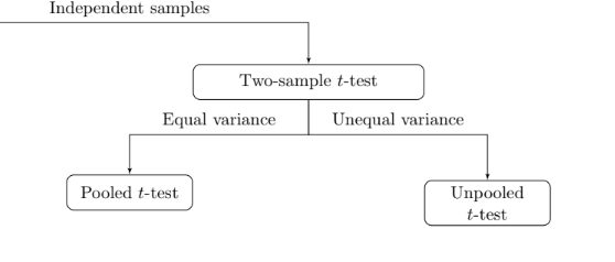
We need to discuss about variance first
$A \sim \mathcal{N}(\mu_A, \sigma^2_A)$, $B \sim \mathcal{N}(\mu_B, \sigma^2_B)$
There are four unknown parameters, the two population means ($\mu_A$ and $\mu_B$) and the two population standard deviations ($\sigma_A$ and $\sigma_B$)
We need to discuss about variance first
If the two sample variances are close enough, we can assume $\sigma_A = \sigma_B$ and perform pooled inference (pooled t-test).
Otherwise, assume $\sigma_A \neq \sigma_B$ and perform unpooled t-test
Hypothesis tesing - $\sigma_A \neq \sigma_B$ or $\sigma_A = \sigma_B$
- First, check the following assumptions:
- Quantitative variables + random sample
- Approximately normal population distributions for each group. This is mainly important for small sample sizes($<30$). Make a graphical display of both samples and check for extreme skew or outliers.
Hypothesis tesing - $\sigma_A \neq \sigma_B$ or $\sigma_A = \sigma_B$
- Second, set up the hypothesis.
or $$ \operatorname{Right\ tail:} H_a: \mu_1-\mu_2 > 0, $$ or $$ \operatorname{Two\ sided:} H_a: \mu_1-\mu_2 \neq 0 $$
Hypothesis tesing - if assume $\sigma_A = \sigma_B$ $\implies$ pooled t-test
Third, compute the test-statistic $t^∗$ through
$$t^* = \frac{(\bar{x}_1 - \bar{x}_2) - 0}{s_p\sqrt{\frac{1}{n_1}+\frac{1}{n_2}}}$$
where $\bar{x}_1$ and $\bar{x}_2$ are the sample mean of 2 groups; $s_1$ and $s_2$ are sample standard deviation of 2 groups, respectively.
$s_p$ is the pooled standard deviation, could be calculated using stat software. $t^*$ follows t-distribution with $df = n_1+n_2-2$.
Hypothesis tesing - if assume $\sigma_A \neq \sigma_B$ $\implies$ unpooled t-test
Third, compute the test-statistic $t^∗$ through
$$t^* = \frac{(\bar{x}_1 - \bar{x}_2) - 0}{\sqrt{\frac{s_1^2}{n_1}+\frac{s_2^2}{n_2}}}$$
where $\bar{x}_1$ and $\bar{x}_2$ are the sample mean of 2 groups; $s_1$ and $s_2$ are sample standard deviation of 2 groups, respectively.
Degree of freedom ($df$) could be obtained using stat software.
Hypothesis tesing - $\sigma_A \neq \sigma_B$ or $\sigma_A \neq \sigma_B$
Fourth step, calculate p-value using statistical software (Stat Crunch, for this course).
Fifth, draw conclusion by comparing the P-value to the significance level α.
- If P-value < $\alpha$, --> reject $H_0$. There is sufficient evidence to support $H_a$ under $\alpha$ significance level.
- If P-value ≥ $\alpha$, --> do not reject $H_0$. There is no sufficient evidence to support $H_a$ under $\alpha$ significance level.
Confidence interval for the population mean difference with independent sample- the recipe
Suppose $\bar{x}_1$ and $\bar{x}_2$ are the sample mean of 2 groups; $s_1$ and $s_2$ are sample standard deviation of 2 groups, respectively.
CI for $ \mu_1 - \mu_2$ is given by
- Degree of freedom should be obtained from stat software.
